Homer GUI
Jump to navigation
Jump to search
- Before running the Matlab HOMER GUI make sure that you have read the Instructions to setup LIBISIS and for both the standalone and matlab versions insure you have read instructions on how to setup the GUI, and acted on them.
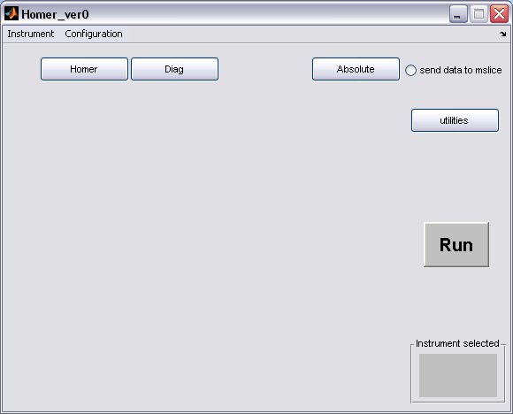
- Homer will start from the matlab command line to bring up a GUI window
>> Homer_ver0

select your instrument using the drop-down menu, this will create the instrument defaults which were defined in the Homer Gui setup

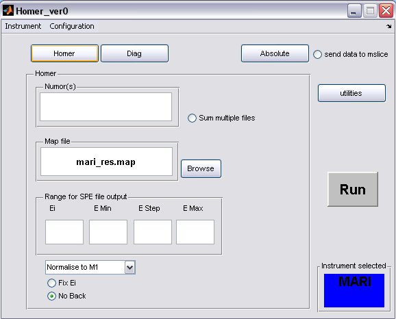
- click on the Homer button to bring up the homer panel

- a) The default map file for the instrument will be filled in, but you can select another one or one you have created using the Map File Format, provided you have placed it in the map file directory.
- b) Fill in energy values for the SPE file output
- c) The Ei will be determined from the run unless the Fix Ei radiobutton is selected
- d) If you want to subtract a flat background from the data then unselect the No Back radiobutton
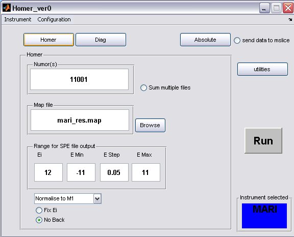
- A completed Homer panel may look something like this...

- a) multiple runs to be treated with the same parameters can be defined using ',' or ':' to denote discrete or continuous run numbers respectively, for example
11001,11004,11006,11010:11015
- b) when homer is running on an instrument analysis machine an updatestore command in the OpenGenie window will create an INST00000.RAW file (where INST=MAP/MAR/MER) and place it in the relevant instrument data folder, therefore to homer an unfinished run type in 00000 in the run number window
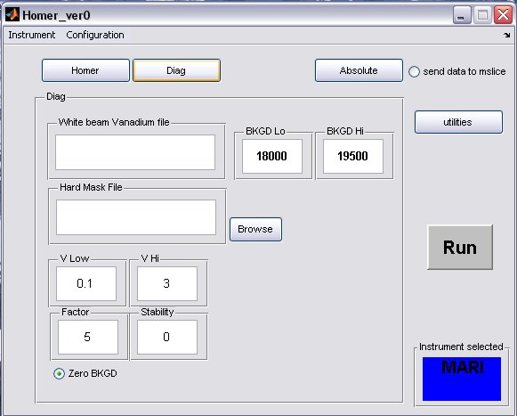
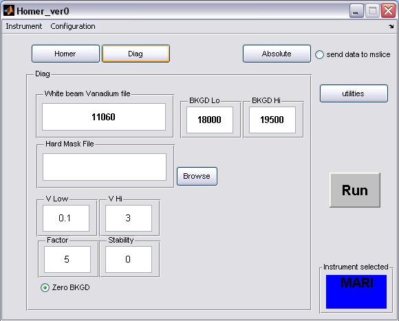
- click on the Diag button to bring up the Diag panel

- a) fill in the white beam run numor, and optionally select a hard mask (if there is one for your instrument)
- b) the background limits can also be changed, if you have selected to perform a flat background subtraction on the homer panel, then these are the limits which will be used
- A completed Diag panel may look something like this...

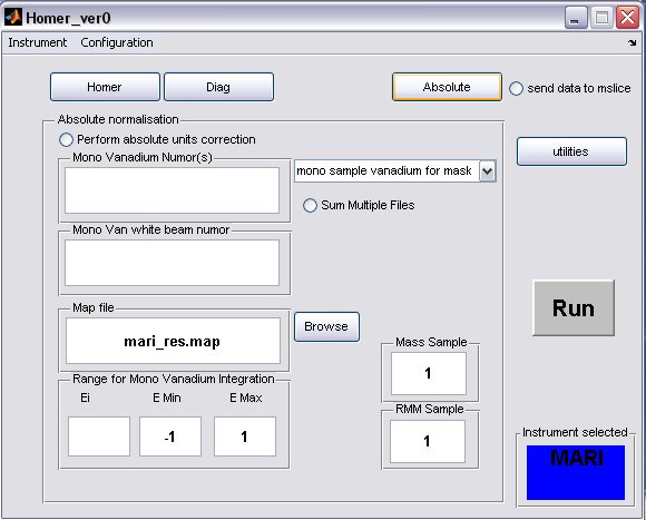
- click on the Absolute button to bring up the Absolute Normalisation panel, absolute normalisation is not selected to be performed by default

- a) Generally the Mono Van white beam numor will be the same as the sample white beam numor, but in special cases for pre PCICP MAPS experiments a diffferent wiring was used for these runs, in this case select the appropriate drop-down menu

and select a different map file.
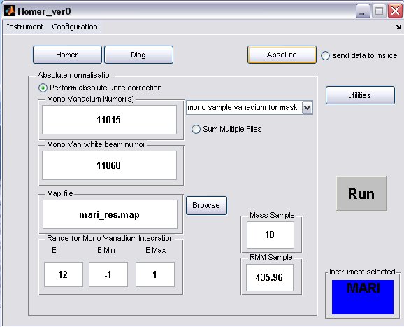
- b) fill in appropriate Sample Mass, Sample RMM and Ei, if the Fix Ei button was selected on the Homer panel, then the energy will be fixed.
- c) select the radiobutton to perform the normalisation
- A completed Diag panel may look something like this...

- Press the Run button to start the homer process. A progress bar will pop up showing what operation is being performed in the sequence.


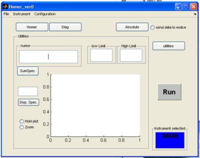
Utilities
- If you click the utilities button a screen appears. Here you can plot single spectra or summed spectra from the selected RAW file.

a) fill in the run number to use for plotting in the numor box
b) pick a low and high limit for summing spectra together and click the sumspec button
OR
c) enter a single spectra and click disp spectra
- Checking hold plot will hold the last plot and make the next plot a different colour
- Checking zoom allows you to zoom in on the plot
- Result of summing spectra 50 to 60 in RAW file 11001 in the same examples given above:

- Result of looking at single spectra 3 in the same RAW file:
